Urban Big Data Analytics
Lecture 9Statistical Modeling
July 30, 2019
Instructor: Andy Hong, PhD
Lead Urban Health Scientist
The George Institute for Global Health
University of Oxford
Assignment 4
- Assignment 4: link
- Any issues? errors?
- Very similar to our group session yesterday
- Due tomorrow (Weds) by 5:00pm
- Send your R code as well
Statistical Learning
What is statistical learning?
- A set of tools for understanding data
- Based on probability and statistics
- Supervised learning: using inputs to estimate outputs
- Unsupervised learning: inputs but no outputs
- Good for explanation
- Linear regression, logistic regreassion, classification
What about machine learning?
- Algorithm-based models
- Supervised and unsupervised learnings
- Good for prediction
- Random forest, support vector machine (SVM), gradient boosting
Statistical Learning vs Machine Learning
| Statistical Learning | Machine Learning |
|---|---|
|
|
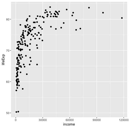
Simple regression
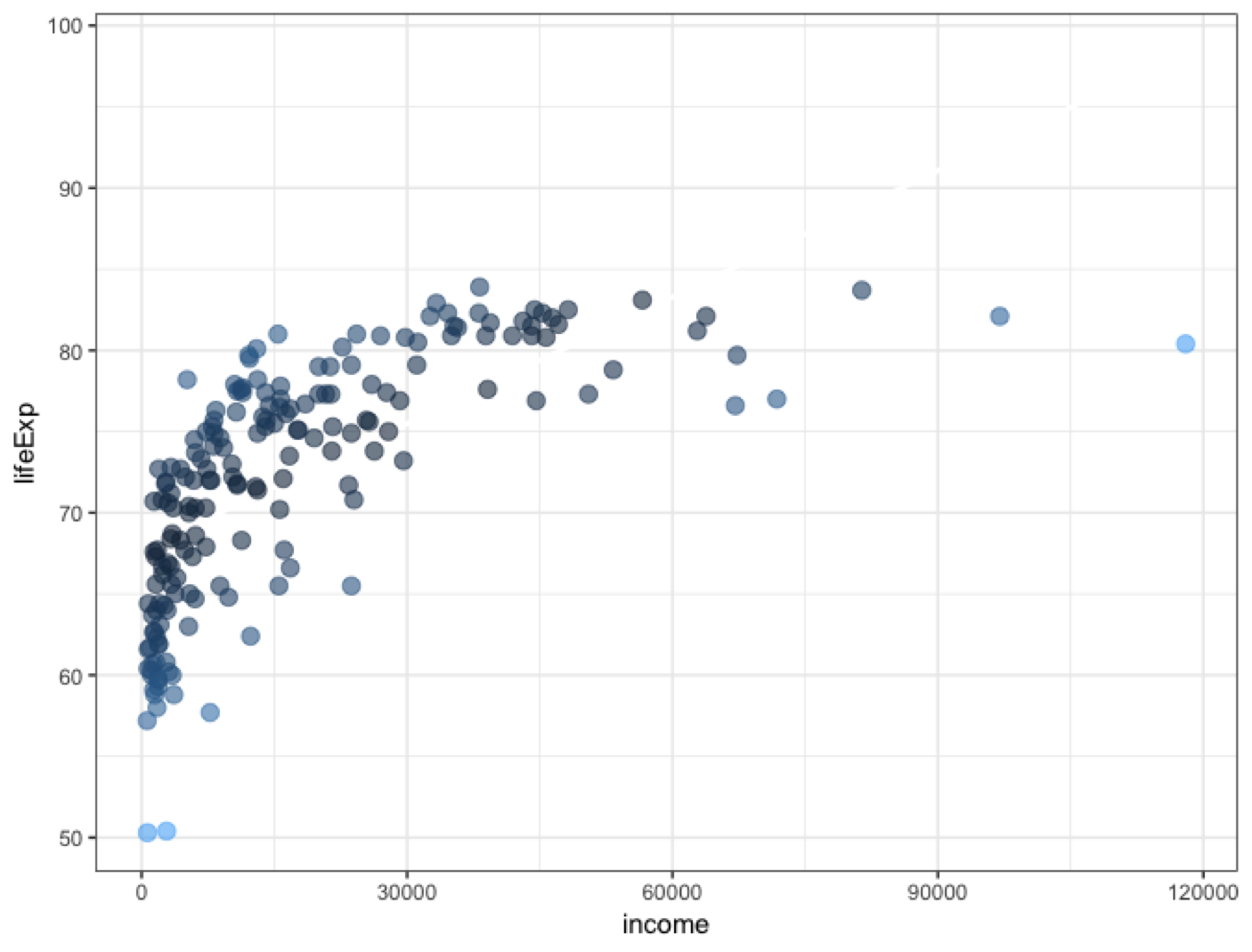
$$ x = income, y = lifeExp $$
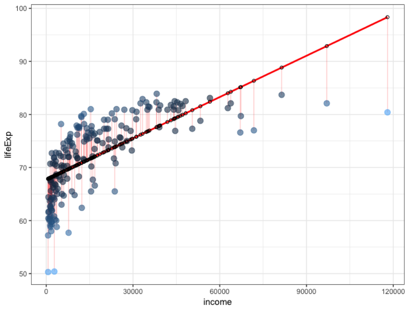
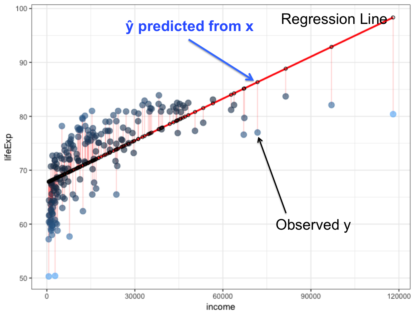
Regression Line
Life expectancy as a function of income
$$ lifeExp \approx f(income) $$
$$ lifeExp = \beta_1 * income + \varepsilon $$
Regression explained
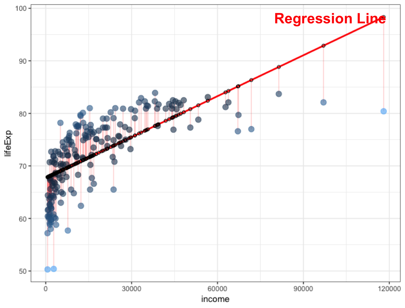
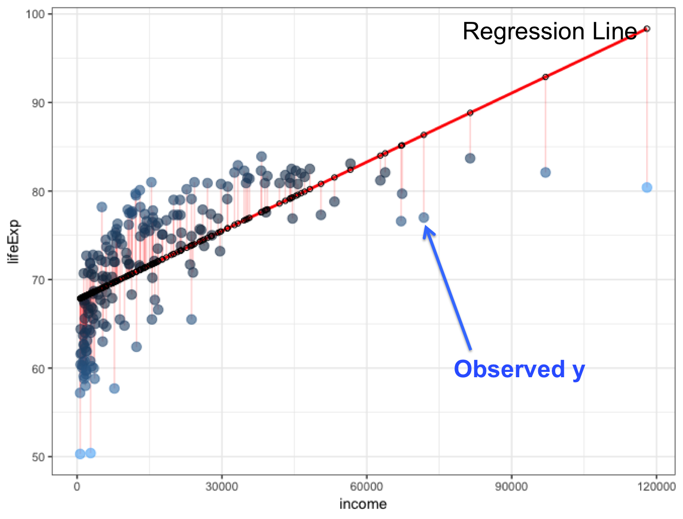
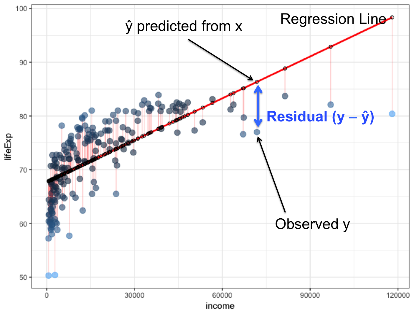
Ordinary Least Squares
Visual explanation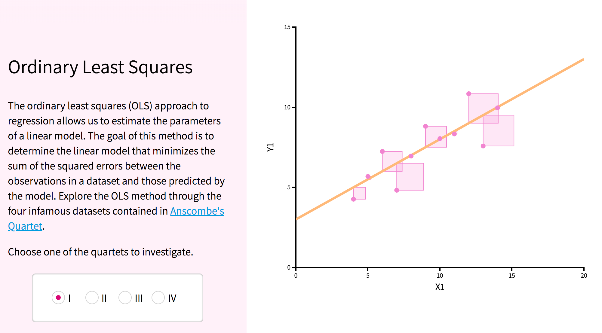
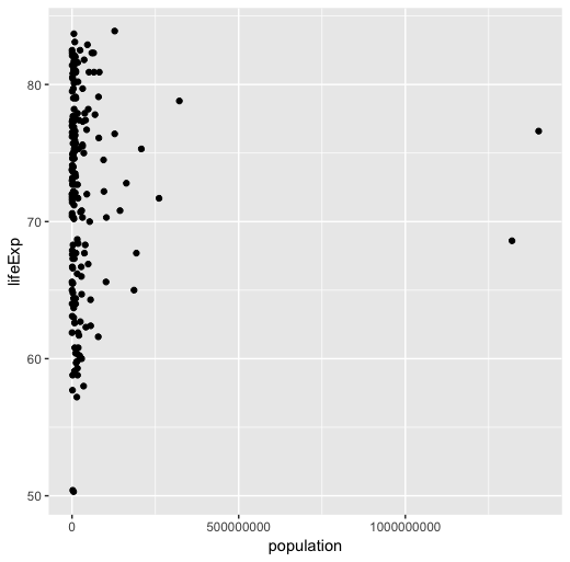
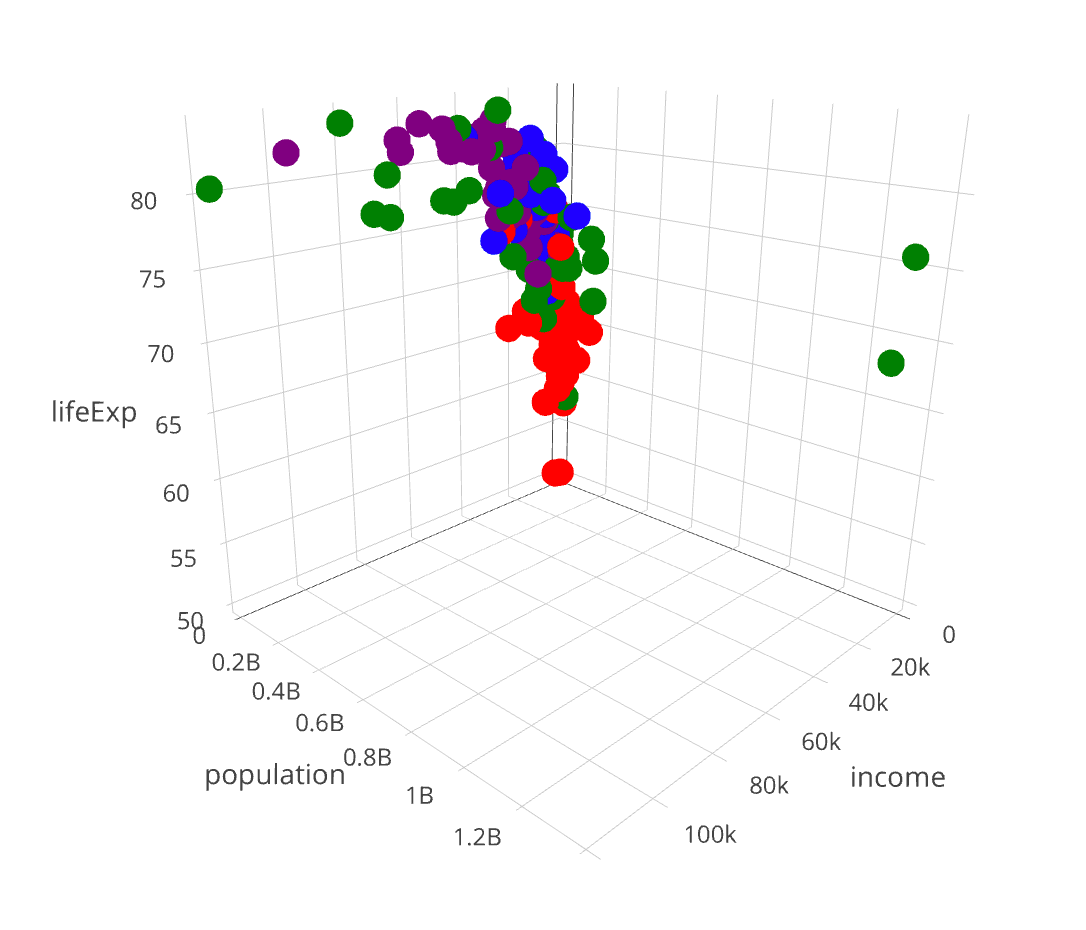
Multiple regression
$$ lifeExp \approx f(income, population) $$
Multiple regression
Simple Regression Demo
					# Simple regression
					m1 = lm(data = gapminder, lifeExp ~ income)
					summary(m1)

					# Call:
					#   lm(formula = lifeExp ~ income, data = gapminder)
					#
					# Residuals:
					#   Min      1Q  Median      3Q     Max
					# -18.032  -3.948   1.314   4.217   9.300
					#
					# Coefficients:
					#   Estimate  Std. Error t value            Pr(>|t|)
					# (Intercept) 67.70194625  0.54603278  123.99 <0.0000000000000002 ***
					#   income       0.00025963  0.00002118   12.26 <0.0000000000000002 ***
					#   ---
					#   Signif. codes:  0 ‘***’ 0.001 ‘**’ 0.01 ‘*’ 0.05 ‘.’ 0.1 ‘ ’ 1
					#
					# Residual standard error: 5.522 on 185 degrees of freedom
					# Multiple R-squared:  0.4482,	Adjusted R-squared:  0.4452
					# F-statistic: 150.3 on 1 and 185 DF,  p-value: < 0.00000000000000022
Multiple Regression demo
				# Multiple regression
				m2 = lm(data = gapminder, lifeExp ~ income + population)
				summary(m2)

				# Call:
				#   lm(formula = lifeExp ~ income + population, data = gapminder)
				#
				# Residuals:
				#   Min      1Q  Median      3Q     Max
				# -17.939  -3.903   1.410   4.129   9.379
				#
				# Coefficients:
				#   Estimate      Std. Error t value            Pr(>|t|)
				# (Intercept) 67.602268543445  0.560501264567 120.610 <0.0000000000000002 ***
				#   income       0.000260247911  0.000021214915  12.267 <0.0000000000000002 ***
				#   population   0.000000002244  0.000000002797   0.802               0.423
				# ---
				#   Signif. codes:  0 ‘***’ 0.001 ‘**’ 0.01 ‘*’ 0.05 ‘.’ 0.1 ‘ ’ 1
				#
				# Residual standard error: 5.528 on 184 degrees of freedom
				# Multiple R-squared:  0.4501,	Adjusted R-squared:  0.4441
				# F-statistic: 75.31 on 2 and 184 DF,  p-value: < 0.00000000000000022